R-language source codes for some papers:
Fitting surface postmortem age-frequency distributions from the mixed layer: Six density functions for fitting parameters of models with optimizing likelihoods are followed by age data of four depth assemblages. Fitting of age data with models occurs within the loop, followed by (1) figures showing the relation between the observed medians and IQRs and the values expected under different models, (2) likelihood surfaces for the Weibull and two-phase model, (3) simulations showing the effect of loss rate on the shape of AFD under one-phase and two-phase models, and (4) simulations showing the effects of sample size and fluctuating sinusoidal production on loss-rate parameters.
Reference for models with variable production and priors: Tomašových A., Kidwell S.M., Foygel Barber R. 2016. Inferring skeletal production from time-averaged assemblages: skeletal loss pulls the timing of production pulses towards the modern period. Paleobiology 42.
Reference for two-phase exponential model: Tomašových A., Kidwell S.M., Foygel Barber R., Kaufman D.S. 2014. Long-term accumulation of carbonate shells reflects a 100-fold drop in loss rate. Geology 42, 9, 819-822.
Range-shuffling null model: (1) Range midpoints are randomly placed on a shelf (along each oceanic margin). (2) Two-dimensional geographic ranges (approximated by a rectangle defined by latitudes and longitudes) are randomly sampled from the frequency distribution of empirical latitudinal ranges along each margin (i.e., the range-shuffling algorithm) and centered on the midpoints. Each empirical latitudinal range has a corresponding longitudinal range that sets the longitudinal dimension of the rectangle. (3) If the northern or southern edge of a given range rectangle falls completely within a continent, the position is discarded and the range midpoint is re-positioned, thus conserving the margin-level empirical distribution of latitudinal range sizes. (4) Species are sampled in those 1° cells that are present in the empirical database. (5) The latitudinal and macroecological thermal ranges are computed for each species.
Coordinates and SST of sampled cells.Rdata
Empirical species ranges.Rdata
Reference: Tomašových A., Jablonski D., Berke S.K., Krug Z.A. And Valentine J.W. 2015. Nonlinear thermal gradients shape broad-scale patterns in geographic range size and can reverse Rapoport's rule. Global Ecology and Biogeography 24, 257-267
Time averaging effects on temporal variation in species composition: simulating time averaging of a fossil assemblage at one location that is connected to regional species pool – metacommunity, assuming neutral dispersal-limited metacommunity dynamics.
Reference: Tomašových A., and Kidwell S.M. 2010. The effects of temporal resolution on species turnover and on testing metacommunity models. American Naturalist 175:587-606
Time averaging effects on spatial variation in species composition: spatially-implicit model simulating multiple locations with fossil assemblages undergoing time averaging simultaneously, all locations are connected with regional species pool – comparable to mainland-island metacommunity model.
Reference: Tomašových A., and Kidwell S.M. 2010. Predicting the effects of increasing temporal scale on species composition, diversity, and rank-abundance distributions. Paleobiology 36:672-695
HMD - the same approach as above but allowing for different numbers of living and death assemblages
Reference: Tomašových A., and Kidwell S.M. 2011. Accounting for the effects of biological variability and temporal autocorrelation in assessing the preservation of species abundance. Paleobiology 37: in press.
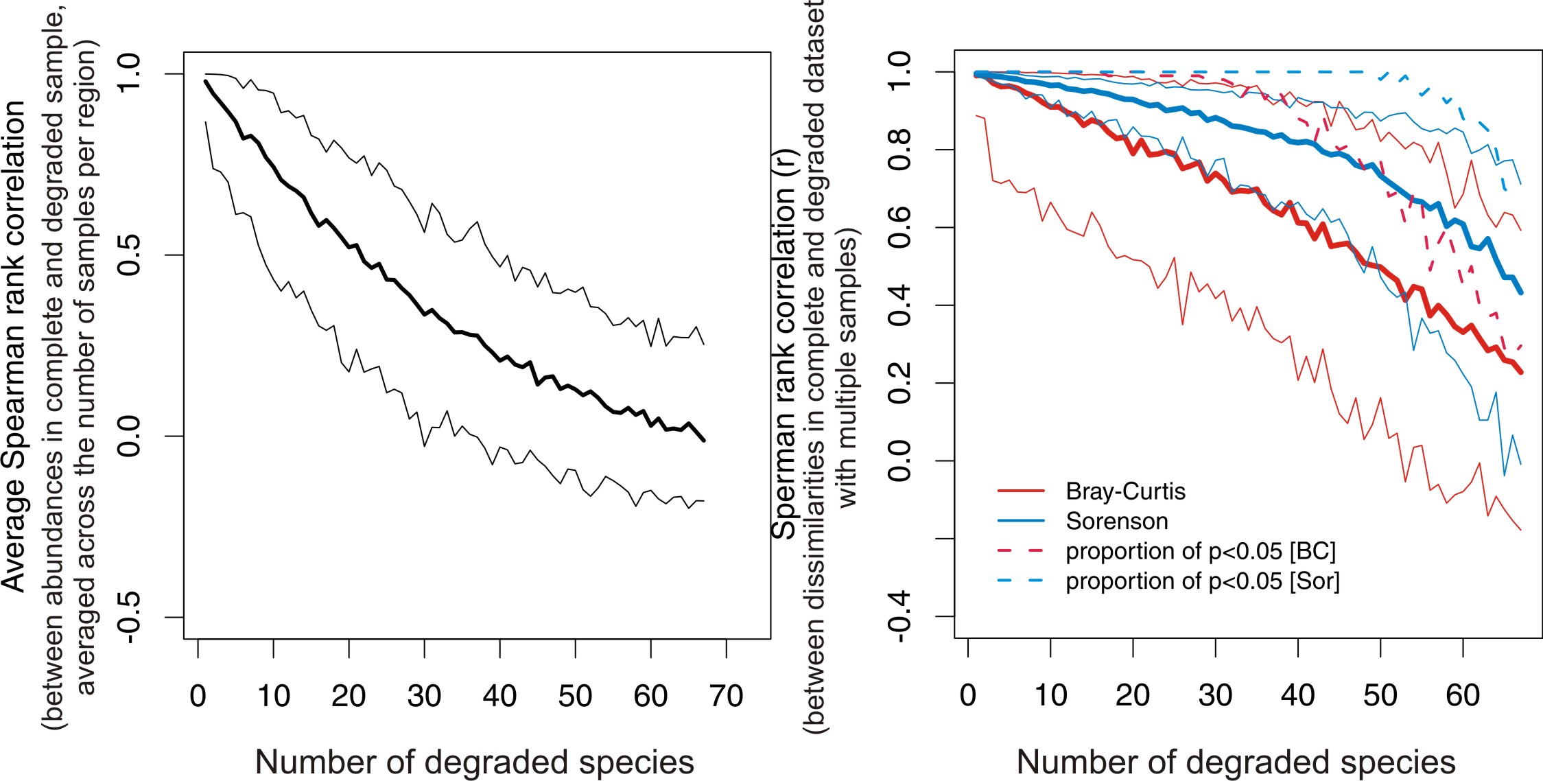
Null expectation for correlation between compositional similarities between complete and degraded samples under random degradation of species: a very simple simulation that recreates figure 8 in Tomasovych and Kidwell 2009. Example file in R format: San Juan Islands
The left figure shows the expected rank correlation between abundances of species in a complete and degraded samples after degradation of 1,2,...N species, using brachiopod-mollusk assemblages from San Juan Islands. The right figure shows the expected rank correlation in between-sample dissimilarities between complete and degraded dataset (p values are from Mantel test). Based on 100 simulation runs. Dashed lines show that even after degradation of many species, Mantel test-based correlations can remain significantly high.
Reference: Tomašových A., and Kidwell S.M. 2009. Preservation of spatial and environmental gradients by death assemblages. Paleobiology 35:122-148